wikilangs/arc

Aramaic - Wikilangs Models

Comprehensive Research Report & Full Ablation Study

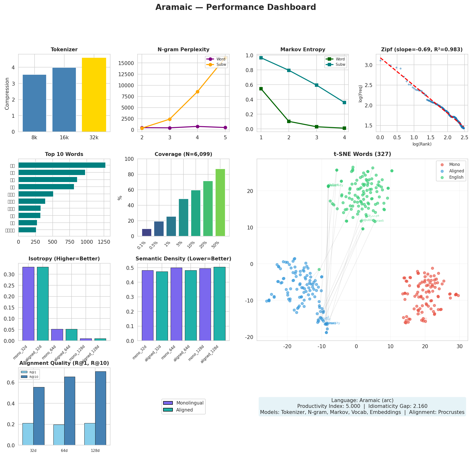
This repository contains NLP models trained and evaluated by Wikilangs, specifically on Aramaic Wikipedia data. We analyze tokenizers, n-gram models, Markov chains, vocabulary statistics, and word embeddings.

📋 Repository Contents

Models & Assets

• Tokenizers (8k, 16k, 32k, 64k)
• N-gram models (2, 3, 4, 5-gram)
• Markov chains (context of 1, 2, 3, 4 and 5)
• Subword N-gram and Markov chains
• Embeddings in various sizes and dimensions (aligned and unaligned)
• Language Vocabulary
• Language Statistics

Analysis and Evaluation

• 1. Tokenizer Evaluation
• 2. N-gram Model Evaluation
• 3. Markov Chain Evaluation
• 4. Vocabulary Analysis
• 5. Word Embeddings Evaluation
• 6. Morphological Analysis (Experimental)
• 7. Summary & Recommendations
• Metrics Glossary
• Visualizations Index

---

1. Tokenizer Evaluation

Results

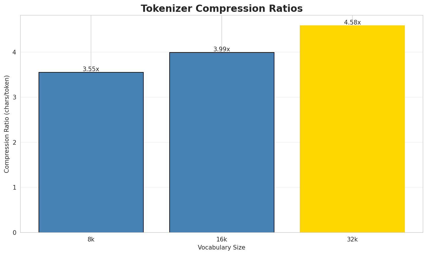
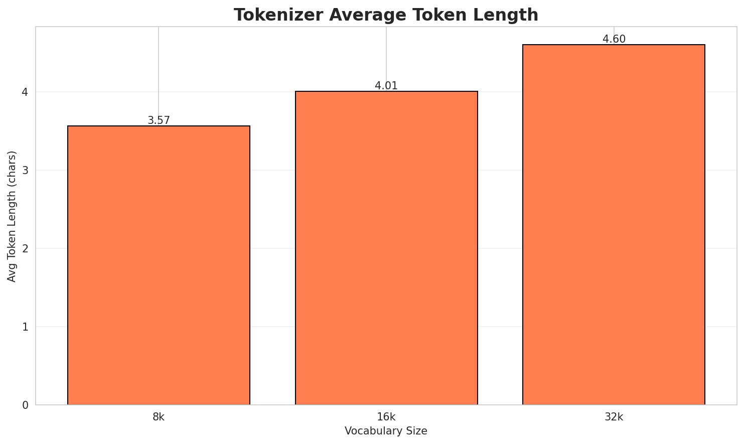
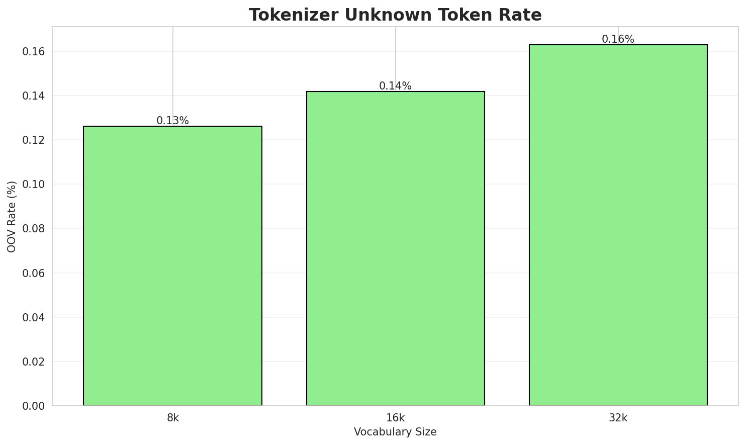
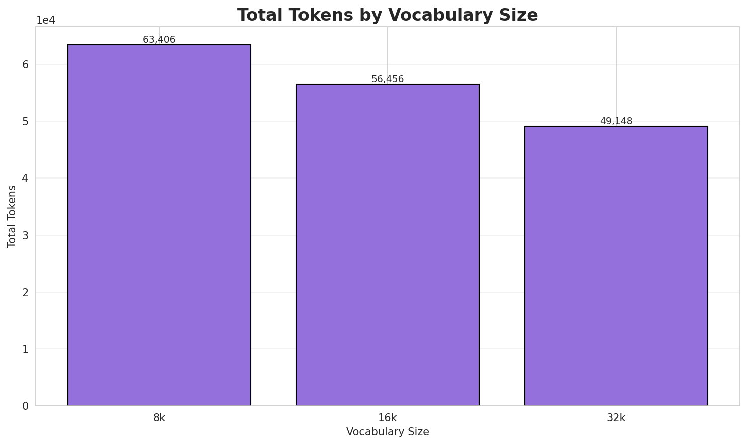
Vocab Size	Compression	Avg Token Len	UNK Rate	Total Tokens
8k	3.553x	3.57	0.1262%	63,406
16k	3.990x	4.01	0.1417%	56,456
32k	4.583x 🏆	4.60	0.1628%	49,148

Tokenization Examples

Below are sample sentences tokenized with each vocabulary size:

Sample 1: ܐܫܬܐ (ܟܢܘܫܝܐ: ܐܫܝ̈ܬܐ) ܗܝ ܡܢܬܐ ܓܠܝܠܬܐ ܕܨܪܘܝܘܬܐ ܕܬܦܠ ܒܒܣܬܪܐ ܕܐܓܢܐ ܕܓܘܫܡ̈ܐ ܕܐܢܫ̈ܐ ܘ...

Vocab	Tokens	Count
8k	▁ܐܫܬܐ ▁( ܟܢܘܫܝܐ : ▁ܐ ܫܝ ̈ܬܐ ) ▁ܗܝ ▁ܡܢܬܐ ... (+20 more)	30
16k	▁ܐܫܬܐ ▁( ܟܢܘܫܝܐ : ▁ܐ ܫܝ ̈ܬܐ ) ▁ܗܝ ▁ܡܢܬܐ ... (+18 more)	28
32k	▁ܐܫܬܐ ▁( ܟܢܘܫܝܐ : ▁ܐܫܝ̈ܬܐ ) ▁ܗܝ ▁ܡܢܬܐ ▁ܓܠܝܠܬܐ ▁ܕܨܪܘܝܘܬܐ ... (+12 more)	22

Sample 2: ܐܫܬܐ ܗܝ ܓܕܫܐ ܐܣܝܝܐ. ܐܫܬܐ ܗܝ ܚܡܝܡܘܬ ܓܘܫܡܐ ܠܥܠ ܡܢ ܫܘܝܐ ܟܝܢܝܐ ܕܚܡܝܡܘܬܐ ܓܘܝܬܐ ܕܓܘܫܡܐ...

Vocab	Tokens	Count
8k	▁ܐܫܬܐ ▁ܗܝ ▁ܓܕܫܐ ▁ܐܣ ܝܝܐ . ▁ܐܫܬܐ ▁ܗܝ ▁ܚܡ ܝܡ ... (+10 more)	20
16k	▁ܐܫܬܐ ▁ܗܝ ▁ܓܕܫܐ ▁ܐܣܝܝܐ . ▁ܐܫܬܐ ▁ܗܝ ▁ܚܡܝܡܘܬ ▁ܓܘܫܡܐ ▁ܠܥܠ ... (+6 more)	16
32k	▁ܐܫܬܐ ▁ܗܝ ▁ܓܕܫܐ ▁ܐܣܝܝܐ . ▁ܐܫܬܐ ▁ܗܝ ▁ܚܡܝܡܘܬ ▁ܓܘܫܡܐ ▁ܠܥܠ ... (+6 more)	16

Sample 3: ܡܪܝ ܢܪܣܝ ܕܒܙ (ܐܬܝܠܕ 17 ܐܝܪ - ܡܝܬ 14 ܫܒܛ ܗܘܐ ܡܝܛܪܦܘܠܝܛܐ ܕܠܒܢܢ ܘܣܘܪܝܐ ܘܟܠܗ̇ ܐܘܪܘܦܐ...

Vocab	Tokens	Count
8k	▁ܡܪܝ ▁ܢܪܣܝ ▁ܕܒܙ ▁( ܐܬܝܠܕ ▁ 1 7 ▁ܐܝܪ ▁- ... (+17 more)	27
16k	▁ܡܪܝ ▁ܢܪܣܝ ▁ܕܒܙ ▁( ܐܬܝܠܕ ▁ 1 7 ▁ܐܝܪ ▁- ... (+17 more)	27
32k	▁ܡܪܝ ▁ܢܪܣܝ ▁ܕܒܙ ▁( ܐܬܝܠܕ ▁ 1 7 ▁ܐܝܪ ▁- ... (+16 more)	26

Key Findings

• Best Compression: 32k achieves 4.583x compression
• Lowest UNK Rate: 8k with 0.1262% unknown tokens
• Trade-off: Larger vocabularies improve compression but increase model size
• Recommendation: 32k vocabulary provides optimal balance for production use

---

2. N-gram Model Evaluation

Results

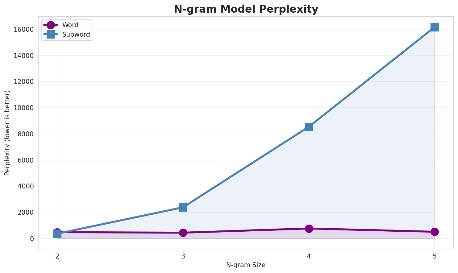
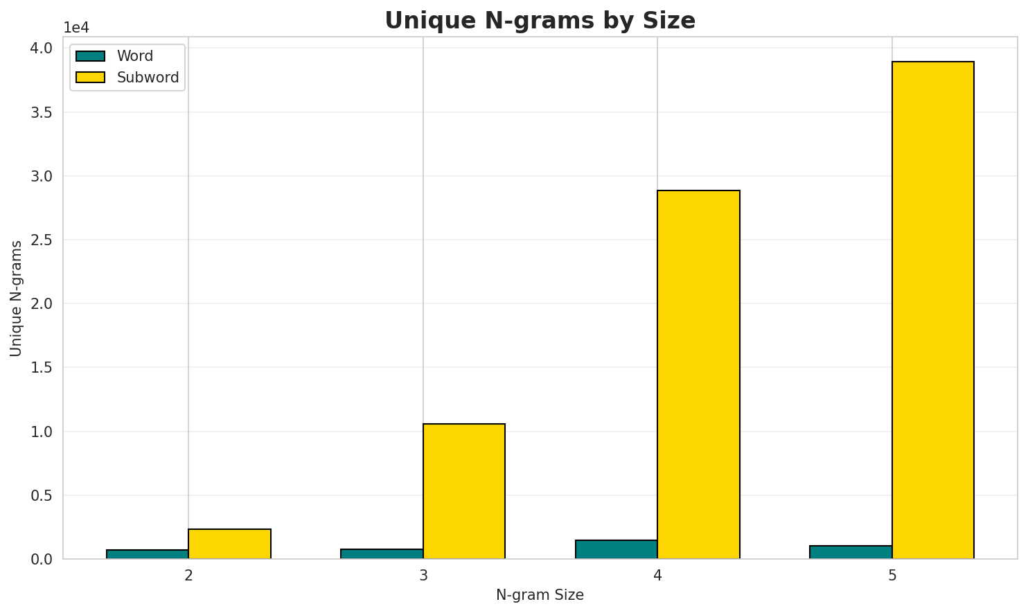
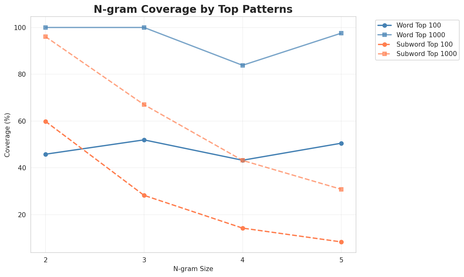
N-gram	Variant	Perplexity	Entropy	Unique N-grams	Top-100 Coverage	Top-1000 Coverage
2-gram	Word	477	8.90	719	45.8%	100.0%
2-gram	Subword	363 🏆	8.50	2,330	59.9%	96.1%
3-gram	Word	438	8.77	754	52.0%	100.0%
3-gram	Subword	2,379	11.22	10,583	28.3%	67.0%
4-gram	Word	759	9.57	1,466	43.3%	83.8%
4-gram	Subword	8,542	13.06	28,872	14.3%	43.2%
5-gram	Word	508	8.99	1,055	50.5%	97.5%
5-gram	Subword	16,168	13.98	38,919	8.4%	30.9%

Top 5 N-grams by Size

2-grams (Word):

Rank	N-gram	Count
1	ܐܦ ܚܙܝ	193
2	ܚܕ ܡܢ	141
3	ܗܝ ܐܬܪܐ	124
4	ܐܝܬ ܠܗ	102
5	ܬܚܘܡܐ ܥܡ	89

3-grams (Word):

Rank	N-gram	Count
1	ܗܘ ܚܕ ܡܢ	72
2	ܟܠܢܚܝܓܐ ܓܐ ܝܢܦܠ	52
3	ܝܠܟܐܒ ܝܓܚܝܐ ܟܠܢܚܝܓܐ	52
4	ܝܢܦܠ ܡܒܤܢ ܐܤܡ	52
5	ܓܐ ܝܢܦܠ ܡܒܤܢ	52

4-grams (Word):

Rank	N-gram	Count
1	ܝܡܓܚܝܢܐ ܐܓܐ ܟܡܠܐ ܣܐܙܬܝܐܢ	52
2	ܝܟܝܟܕ ܝܡܓܚܝܢܐ ܐܓܐ ܟܡܠܐ	52
3	ܢܝܛܠܐ ܝܟܝܟܕ ܝܡܓܚܝܢܐ ܐܓܐ	52
4	ܟܢܫܙܢ ܢܝܛܠܐ ܝܟܝܟܕ ܝܡܓܚܝܢܐ	52
5	ܣܢܝܓܚܝܢܪܢ ܟܢܫܙܢ ܢܝܛܠܐ ܝܟܝܟܕ	52

5-grams (Word):

Rank	N-gram	Count
1	ܝܠܟܐܒ ܝܓܚܝܐ ܟܠܢܚܝܓܐ ܓܐ ܝܢܦܠ	52
2	ܟܠܢܚܝܓܐ ܓܐ ܝܢܦܠ ܡܒܤܢ ܐܤܡ	52
3	ܓܐ ܝܢܦܠ ܡܒܤܢ ܐܤܡ ܟܛܠ	52
4	ܡܒܤܢ ܐܤܡ ܟܛܠ ܚܢܝܬܝܐ ܡܕܛܚܝܢܐ	52
5	ܝܢܦܠ ܡܒܤܢ ܐܤܡ ܟܛܠ ܚܢܝܬܝܐ	52

2-grams (Subword):

Rank	N-gram	Count
1	ܐ _	24,552
2	_ ܕ	7,580
3	ܬ ܐ	7,166
4	_ ܐ	6,890
5	ܝ ܐ	5,689

3-grams (Subword):

Rank	N-gram	Count
1	ܐ _ ܕ	6,099
2	ܬ ܐ _	5,875
3	ܝ ܐ _	4,233
4	ܐ _ ܐ	2,477
5	ܐ _ ܘ	2,392

4-grams (Subword):

Rank	N-gram	Count
1	ܬ ܐ _ ܕ	1,993
2	ܝ ܬ ܐ _	1,513
3	ܐ ܝ ܬ _	1,372
4	ܘ ܬ ܐ _	1,304
5	_ ܡ ܢ _	1,203

5-grams (Subword):

Rank	N-gram	Count
1	ܐ _ ܐ ܘ _	603
2	ܘ ܬ ܐ _ ܕ	543
3	ܐ _ ܡ ܢ _	533
4	_ ܐ ܝ ܬ _	503
5	ܝ ܘ ܬ ܐ _	487

Key Findings

• Best Perplexity: 2-gram (subword) with 363
• Entropy Trend: Decreases with larger n-grams (more predictable)
• Coverage: Top-1000 patterns cover ~31% of corpus
• Recommendation: 4-gram or 5-gram for best predictive performance

---

3. Markov Chain Evaluation

Results

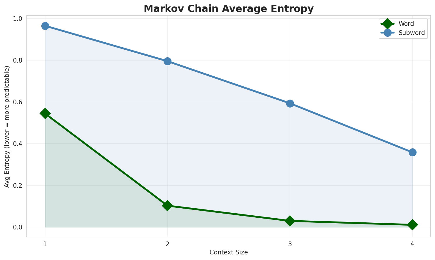
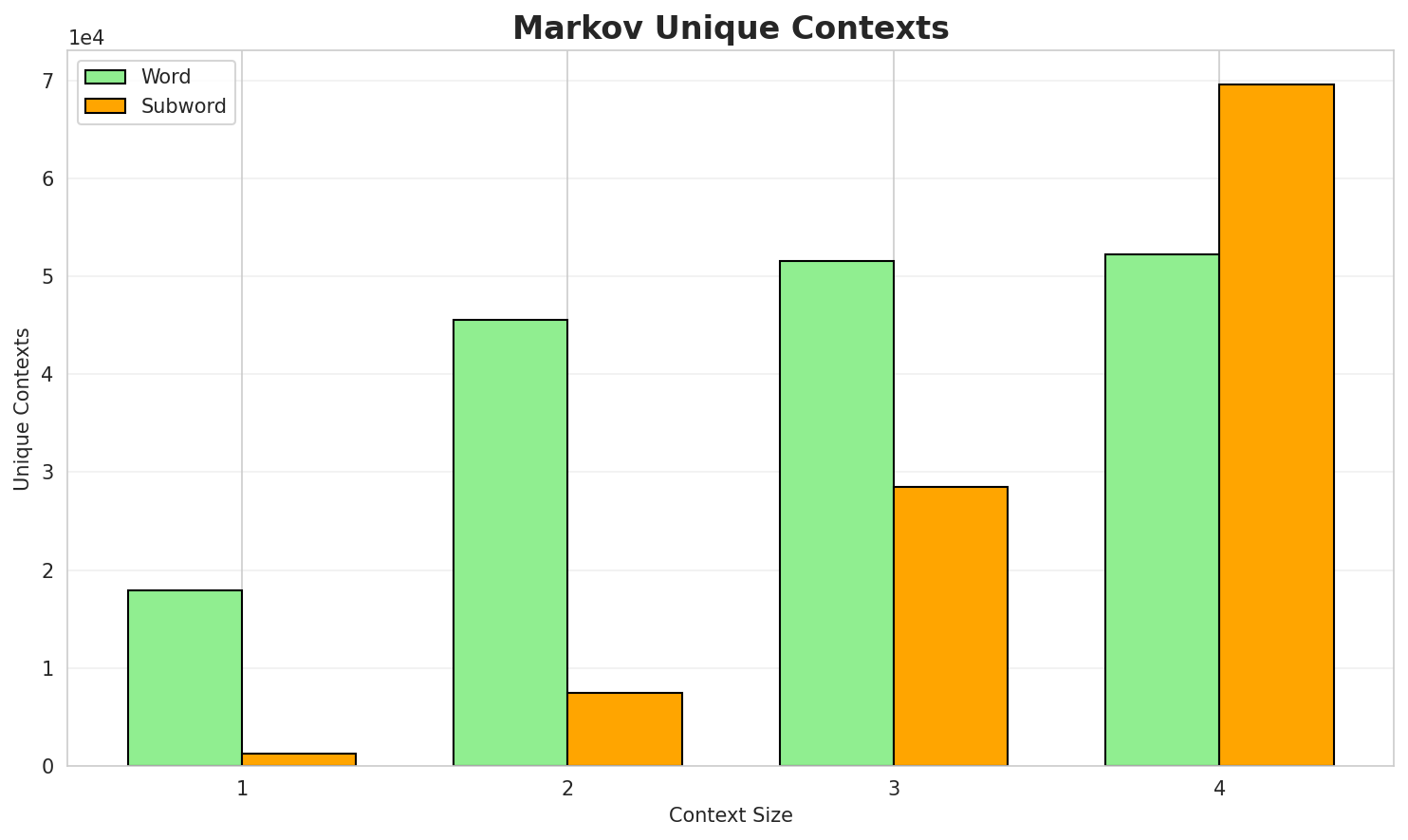
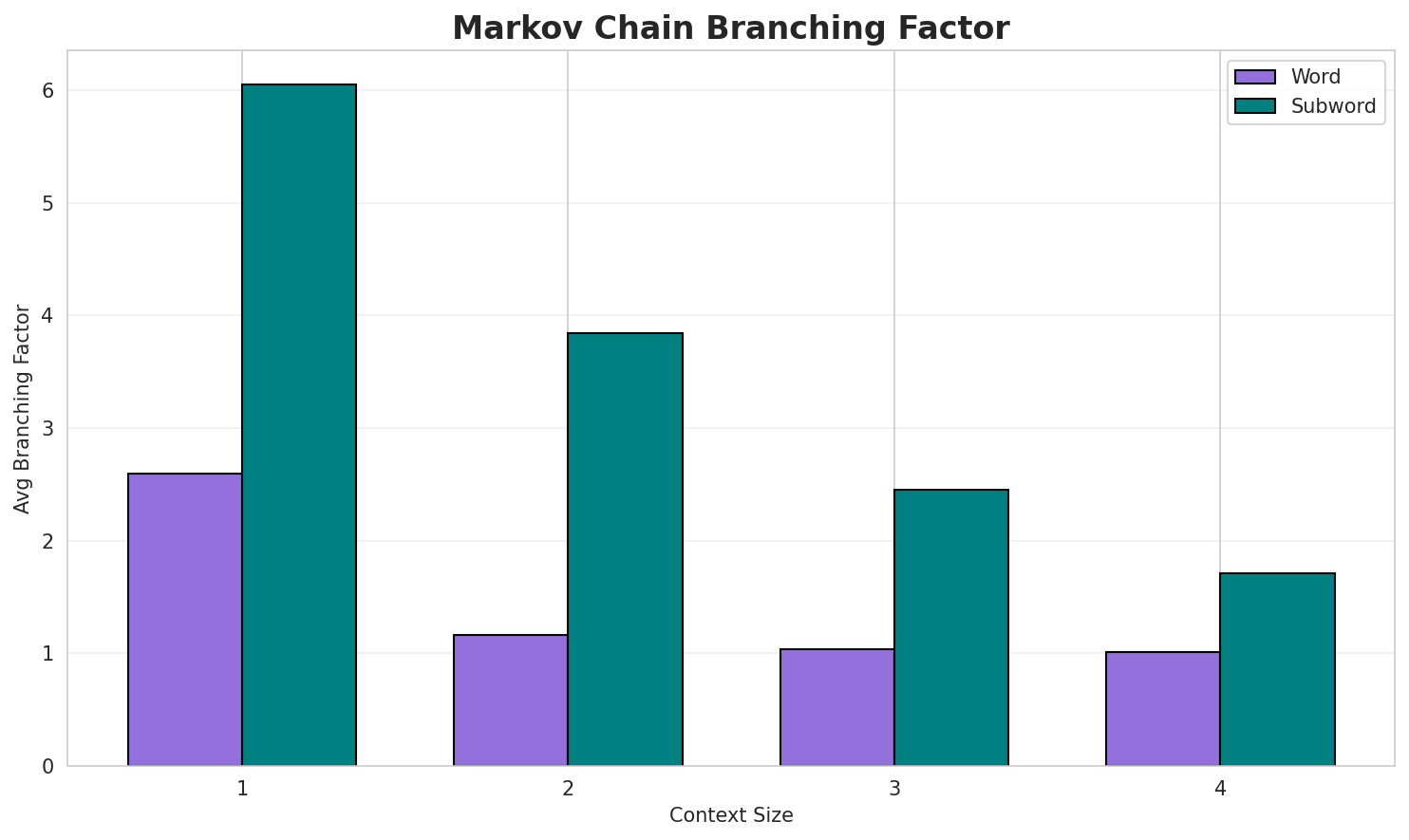
Context	Variant	Avg Entropy	Perplexity	Branching Factor	Unique Contexts	Predictability
1	Word	0.5444	1.458	2.59	17,962	45.6%
1	Subword	0.9651	1.952	6.05	1,231	3.5%
2	Word	0.1025	1.074	1.16	45,549	89.7%
2	Subword	0.7954	1.736	3.84	7,433	20.5%
3	Word	0.0296	1.021	1.04	51,591	97.0%
3	Subword	0.5935	1.509	2.45	28,465	40.7%
4	Word	0.0106 🏆	1.007	1.01	52,240	98.9%
4	Subword	0.3585	1.282	1.71	69,540	64.2%

Generated Text Samples (Word-based)

Below are text samples generated from each word-based Markov chain model:

Context Size 1:

1. ܡܢ ܕܝܪܐ ܕܡܪܝ ܓܒܪܐܝܠ ܗܘ ܫܡܐ ܕܒܗܘ ܢܬܝܕܥܘܢ ܗܘܘ ܡܠܘܢ ܕܝܢ ܪ̈ܥܘܬܐ ܕܝܠܗܘܢ ܒܪܓܘܠܐ ܕܓܗܢܐ ܗܢܐ
2. ܐܘ ܡܣܐܢܐ ܐܘ ܚܡܗܐ ܗܘ ܣܦܪܐ ܕܗܘܫܥ ܘܕܐܫܥܝܐ ܘܗܘܝܘ ܦܪܝܣܐ ܩܘܢܣܛܢܛܝܢ
3. ܗܘ ܢܒܝܐ ܙܥܘܪܐ ܒܠܒܘܫܐ ܕܒܗ ܫܩܠܘ ܐܢܛܝܘܟܝܐ ܘܫܚܠܦ ܗܘܐ ܦܛܪܝܪܟܐ ܩܢܘܢܝܐ ܣܕܪܐ ܘܟܠ ܕܡܘ 2 ܒܢܝܣܢ

Context Size 2:

1. ܐܦ ܚܙܝ ܥܡܐ ܒܝܬܝܘܬܐ de verwandtschaftsbeziehung onkel und tante
2. ܚܕ ܡܢ ܬܪܥܣܪ ܢܒܝ̈ܐ ܙܥܘܪ̈ܐ ܕܬܢܟ ܘܕܕܝܬܝܩܝ ܥܬܝܩܬܐ ܥܬܝܩܬܐ
3. ܗܝ ܐܬܪܐ ܒܐܣܝܐ ܨܝܢ ܐܝܬ ܠܗ̇ ܪܡܙܐ ܕܡܘܠܕܐ ܬܪܝܢܐ ܒܝܕ ܡܝ̈ܐ ܘܪܘܚܐ ܕܩܘܕܫܐ ܝܫܘܥ ܐܡܪ ܠܗ ܘܠܐܚܗ

Context Size 3:

1. ܗܘ ܚܕ ܡܢ ܠܫܢ̈ܐ ܨܝܢܝ̈ܐ ܕܢܬܡܠܠܘܢ ܒܬܝܡܢ ܡܕܢܚ ܕܨܝܢ ܐܝܬܘܗܝ ܠܫܢܐ ܐܡܗܝܐ ܕܝܬܝܪ ܡܢ 90 ܡܠܝܘܢܐ ܐܢܫ̈ܝܢ ܪܝܫܐܝܬ
2. ܢܝܛܠܐ ܝܟܝܟܕ ܝܡܓܚܝܢܐ ܐܓܐ ܟܡܠܐ ܣܐܙܬܝܐܢ ܝܠܟܐܒ ܝܓܚܝܐ ܟܠܢܚܝܓܐ ܓܐ ܝܢܦܠ ܡܒܤܢ ܐܤܡ ܟܛܠ ܚܢܝܬܝܐ ܡܕܛܚܝܢܐ ܡܒܕ ܫܐܢ...
3. ܟܛܠ ܚܢܝܬܝܐ ܡܕܛܚܝܢܐ ܡܒܕ ܫܐܢܡܝܢ ܪܡܝܚܢܐܢ ܢܕܢܐ ܡܠܝܝܐ ܢܟܓܐܝܚܢܛܟ‍ ܟ‍ܝܣܢܐ ܡܓܝܡܡ ܡܟܒܡ ܠܣܐܟ ܒܟܡ ܣܢܝܓܚܝܢܪܢ ܟܢܫ...

Context Size 4:

1. ܝܓܚܝܐ ܟܠܢܚܝܓܐ ܓܐ ܝܢܦܠ ܡܒܤܢ ܐܤܡ ܟܛܠ ܚܢܝܬܝܐ ܡܕܛܚܝܢܐ ܡܒܕ ܫܐܢܡܝܢ ܪܡܝܚܢܐܢ ܢܕܢܐ ܡܠܝܝܐ ܢܟܓܐܝܚܢܛܟ‍ ܟ‍ܝܣܢܐ ܡܓ...
2. ܚܢܝܬܝܐ ܡܕܛܚܝܢܐ ܡܒܕ ܫܐܢܡܝܢ ܪܡܝܚܢܐܢ ܢܕܢܐ ܡܠܝܝܐ ܢܟܓܐܝܚܢܛܟ‍ ܟ‍ܝܣܢܐ ܡܓܝܡܡ ܡܟܒܡ ܠܣܐܟ ܒܟܡ ܣܢܝܓܚܝܢܪܢ ܟܢܫܙܢ ܢ...
3. ܟܛܠ ܚܢܝܬܝܐ ܡܕܛܚܝܢܐ ܡܒܕ ܫܐܢܡܝܢ ܪܡܝܚܢܐܢ ܢܕܢܐ ܡܠܝܝܐ ܢܟܓܐܝܚܢܛܟ‍ ܟ‍ܝܣܢܐ ܡܓܝܡܡ ܡܟܒܡ ܠܣܐܟ ܒܟܡ ܣܢܝܓܚܝܢܪܢ ܟܢܫ...

Generated Text Samples (Subword-based)

Below are text samples generated from each subword-based Markov chain model:

Context Size 1:

1. _ܥܪ_ܙܥܠܐܡܘܦܐܘܗ_ܡ
2. ܐܣܬܐ_ܒܕ_ܐ_ܡܐ_ܕܡܦ
3. ܝܓܝܛܠܚܕܢܪܝܦܝ̈ܘܪܝܐ

Context Size 2:

1. ܐ_ܫܡܐ_ܕܢܐܡܪܝܬ_800
2. _ܕܠܐܬܘܕܝܫܐ_ܘܒܝܬ_ا
3. ܬܐ_ܕܛܚܝܬ_ܡܚܝܬ_ܡܥܘ

Context Size 3:

1. ܐ_ܕܐܬܥܢܘܬܐ_ܠܫܢܐ_(r
2. ܬܐ_ܥܪܒܐ_ܩܘܛܢܝܘܬܐ_ܛ
3. ܝܐ_ܒܪ_ܒܪ_ܐܘ_ܐܘܢܛܐܪ

Context Size 4:

1. ܬܐ_ܕܢܒܥ_ܡܫܝܚܐ._ܥܠܠܢ̈
2. ܝܬܐ_ܕܪ̈ܗܘܡܝܐ܀_ܢܗܪܝܢ܁
3. ܐܝܬ_ܚܡܫܐ_ܨܒܝܢܗ._ܟܬܒ

Key Findings

• Best Predictability: Context-4 (word) with 98.9% predictability
• Branching Factor: Decreases with context size (more deterministic)
• Memory Trade-off: Larger contexts require more storage (69,540 contexts)
• Recommendation: Context-3 or Context-4 for text generation

---

4. Vocabulary Analysis

Statistics

Metric	Value
Vocabulary Size	6,099
Total Tokens	50,661
Mean Frequency	8.31
Median Frequency	3
Frequency Std Dev	32.05

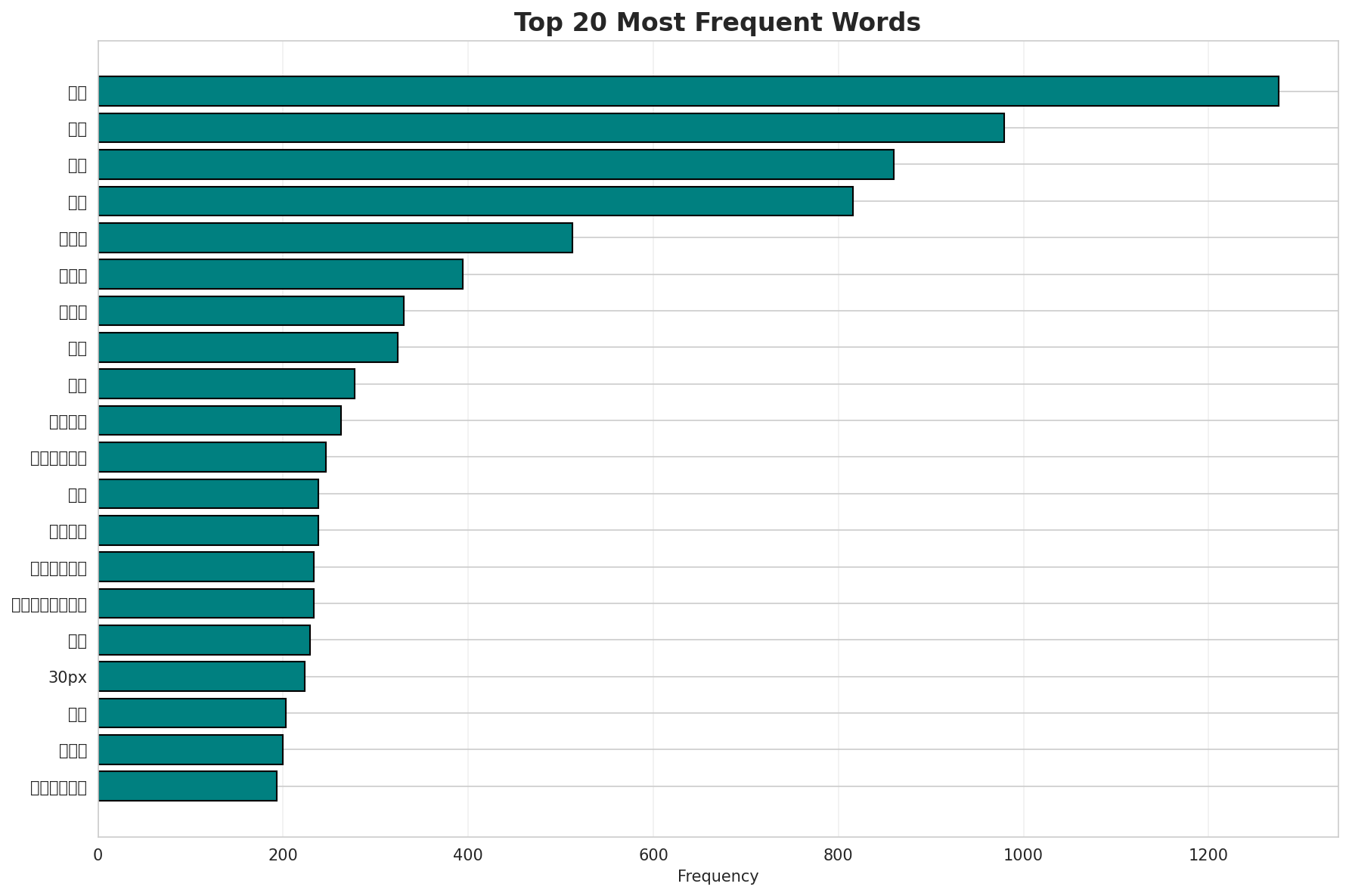
Most Common Words

Rank	Word	Frequency
1	ܡܢ	1,276
2	ܐܘ	979
3	ܗܘ	860
4	ܗܝ	816
5	ܐܝܬ	513
6	ܗܘܐ	394
7	ܘܥܡ	330
8	ܥܠ	324
9	ܐܦ	277
10	ܠܫܢܐ	263

Least Common Words (from vocabulary)

Rank	Word	Frequency
1	ܐܚܹܪ̈ܢܹܐ	2
2	ܦܘܼܪܡܘܼܠܵܐ	2
3	ܢܣܲܒܪܲܚ	2
4	ܚܲܕ	2
5	ܐܘܟܝܬܐ	2
6	ܕܫܠܝܼܡܵܐ	2
7	ܡܚܲܝܕܵܐ	2
8	ܓܵܪܹܫ	2
9	ܕܠܥܸܠ	2
10	ܕܒܘܿܠܨܡܲܢ	2

Zipf's Law Analysis

Metric	Value
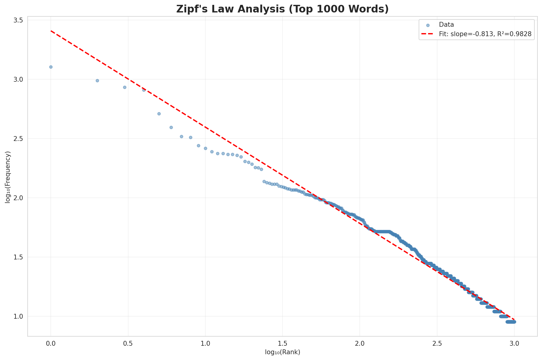
Zipf Coefficient	0.8942
R² (Goodness of Fit)	0.982775
Adherence Quality	excellent

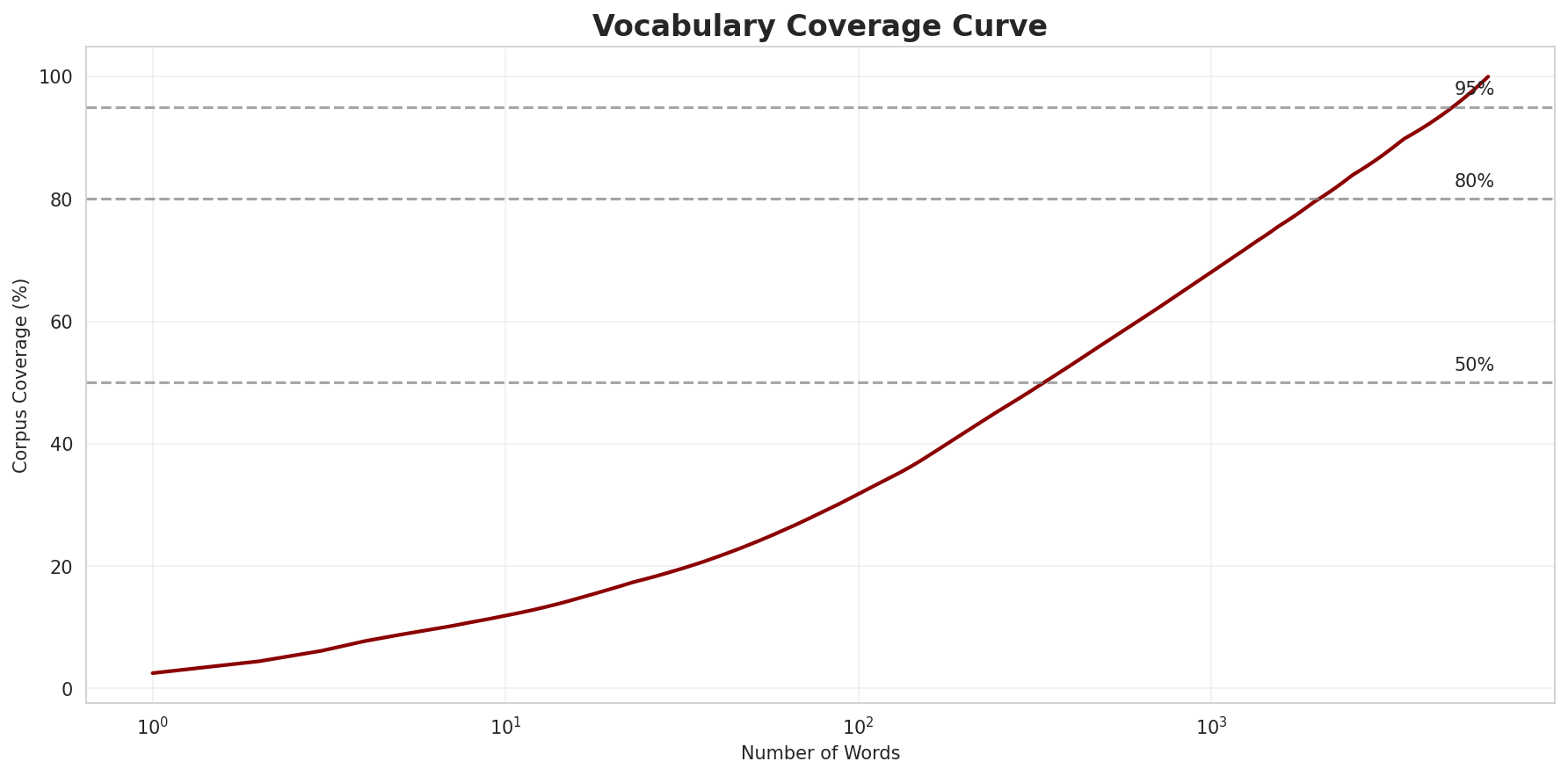
Coverage Analysis

Top N Words	Coverage
Top 100	31.8%
Top 1,000	68.0%
Top 5,000	95.7%
Top 10,000	0.0%

Key Findings

• Zipf Compliance: R²=0.9828 indicates excellent adherence to Zipf's law
• High Frequency Dominance: Top 100 words cover 31.8% of corpus
• Long Tail: -3,901 words needed for remaining 100.0% coverage

---

5. Word Embeddings Evaluation

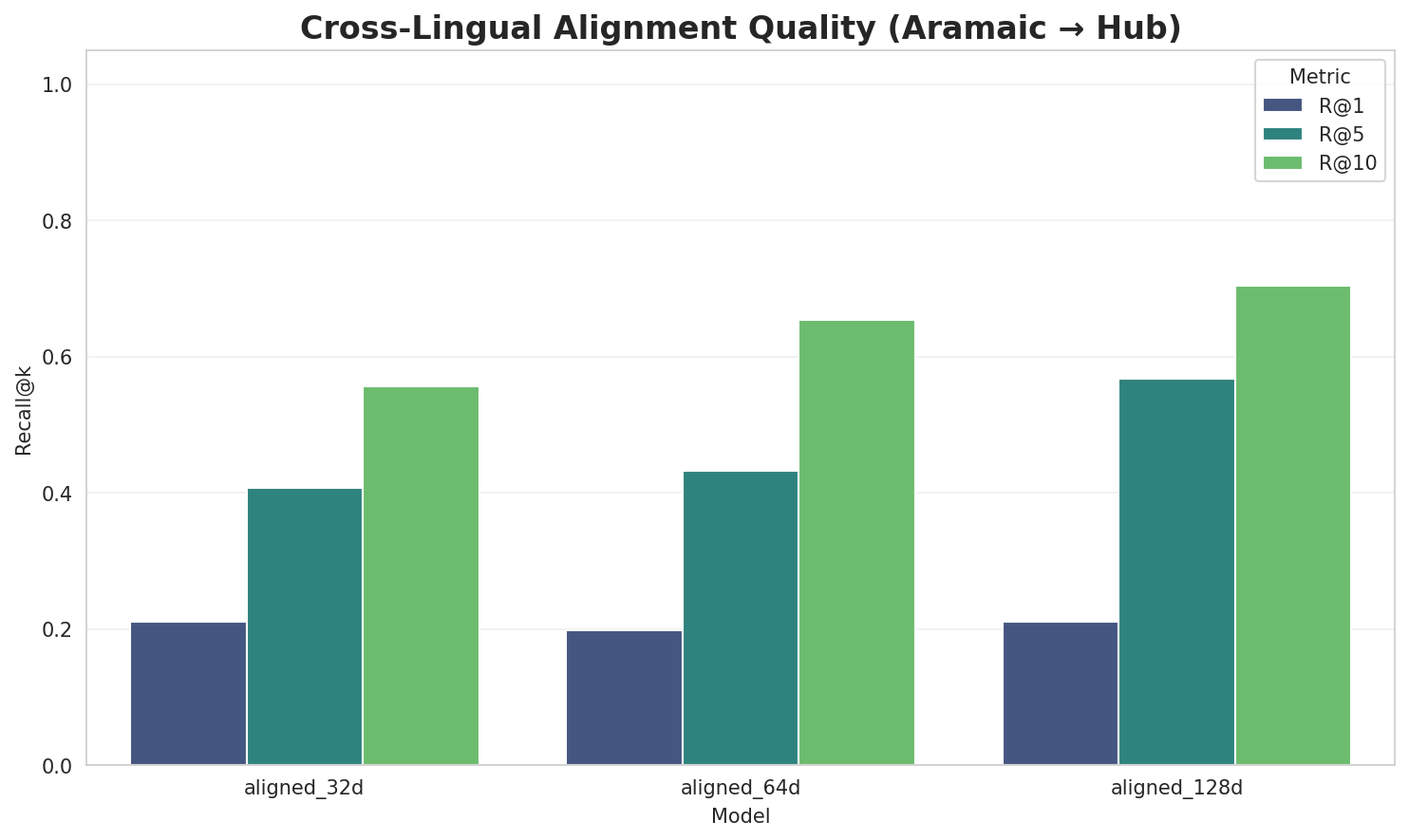
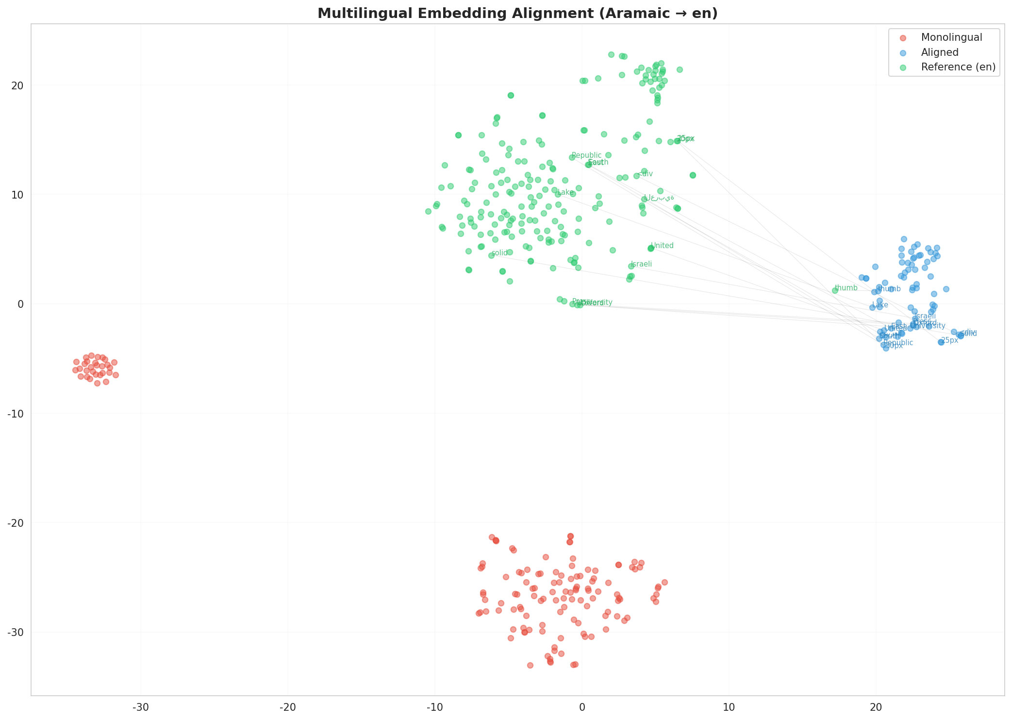
5.1 Cross-Lingual Alignment

5.2 Model Comparison

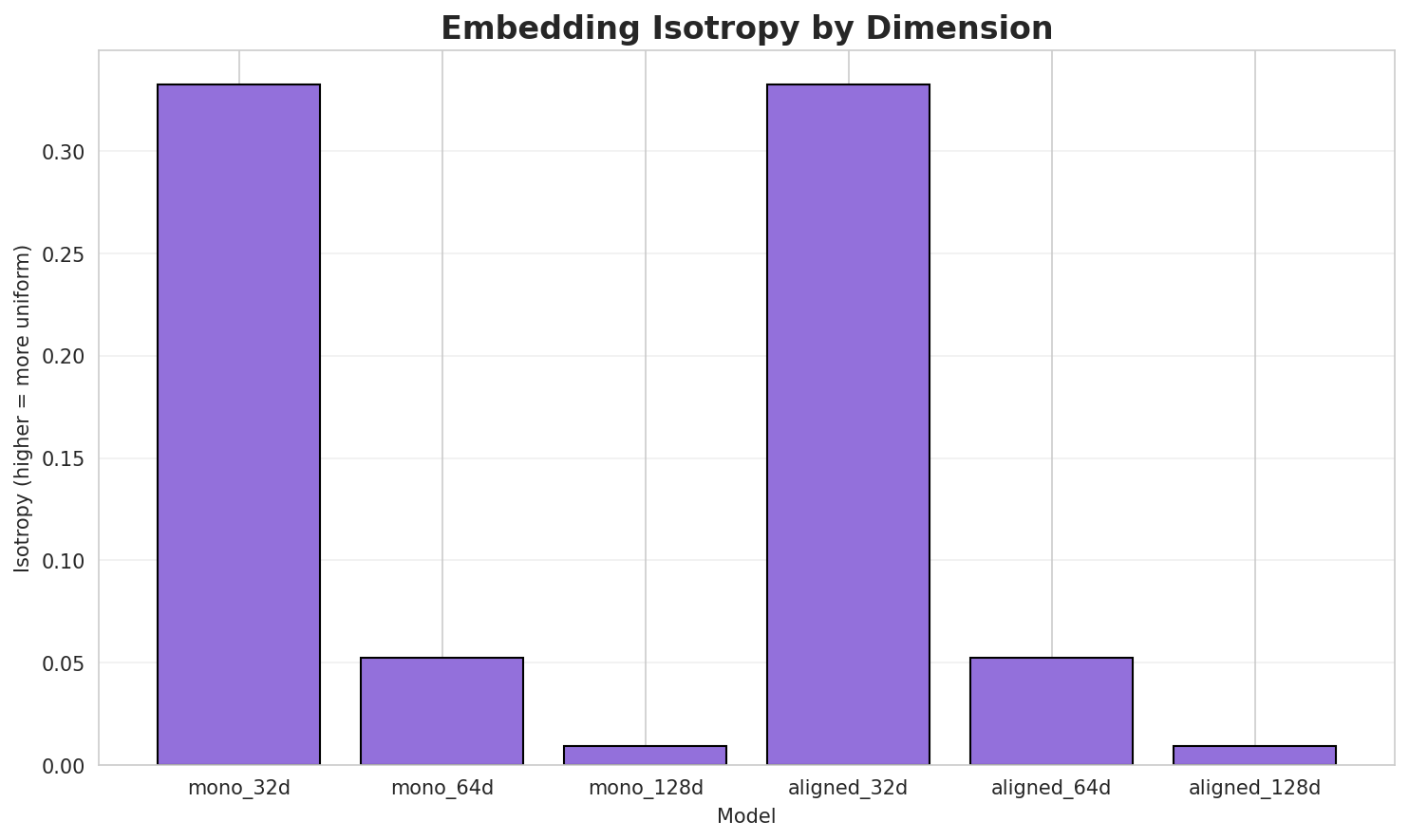
Model	Dimension	Isotropy	Semantic Density	Alignment R@1	Alignment R@10
mono_32d	32	0.3326	0.4816	N/A	N/A
mono_64d	64	0.0524	0.4997	N/A	N/A
mono_128d	128	0.0094	0.4954	N/A	N/A
aligned_32d	32	0.3326 🏆	0.4744	0.2099	0.5556
aligned_64d	64	0.0524	0.4826	0.1975	0.6543
aligned_128d	128	0.0094	0.5048	0.2099	0.7037

Key Findings

• Best Isotropy: aligned_32d with 0.3326 (more uniform distribution)
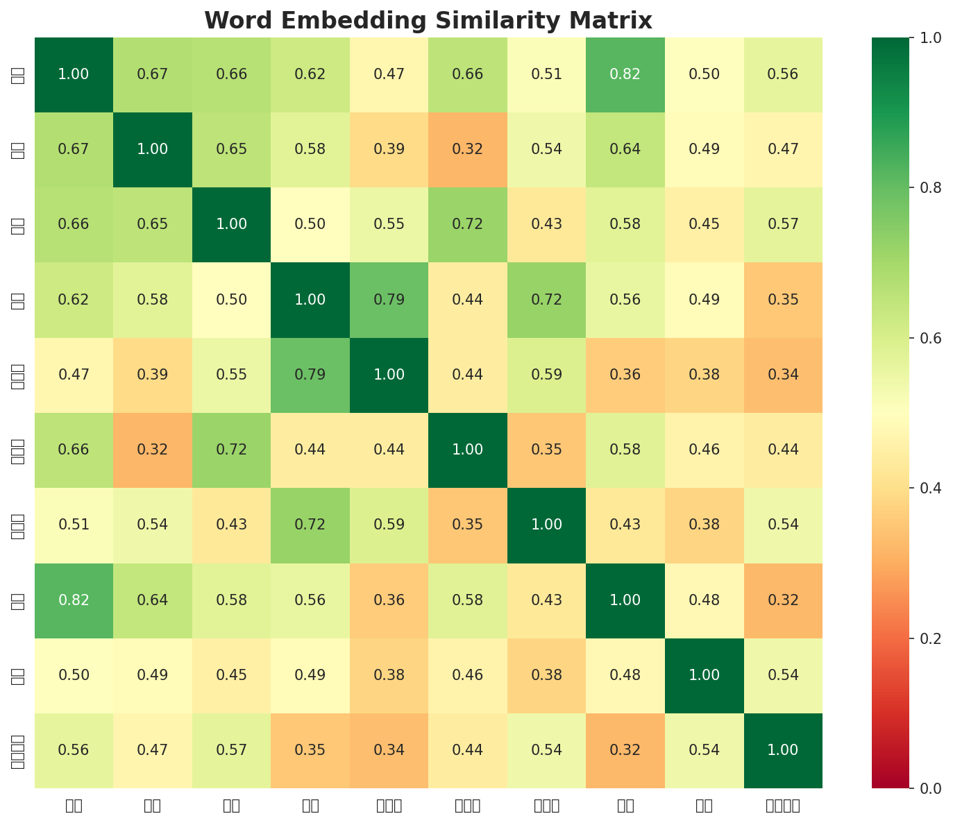
• Semantic Density: Average pairwise similarity of 0.4897. Lower values indicate better semantic separation.
• Alignment Quality: Aligned models achieve up to 21.0% R@1 in cross-lingual retrieval.
• Recommendation: 128d aligned for best cross-lingual performance

---

6. Morphological Analysis (Experimental)

This section presents an automated morphological analysis derived from the statistical divergence between word-level and subword-level models. By analyzing where subword predictability spikes and where word-level coverage fails, we can infer linguistic structures without supervised data.

6.1 Productivity & Complexity

Metric	Value	Interpretation	Recommendation
Productivity Index	5.000	High morphological productivity	Reliable analysis
Idiomaticity Gap	2.160	High formulaic/idiomatic content	-

6.2 Affix Inventory (Productive Units)

These are the most productive prefixes and suffixes identified by sampling the vocabulary for global substitutability patterns. A unit is considered an affix if stripping it leaves a valid stem that appears in other contexts.

Productive Prefixes

Prefix	Examples

Productive Suffixes

Suffix	Examples
-ܐ	ܬܫܐܢܐܟܐܠܐ, ܟܘܕܢܝܐ, ܕܚܘܼܡܵܐ
-ܬܐ	ܐܒܪ̈ܗܡܝܬܐ, ܕܡܥܡܕܝܬܐ, ܫܬܐ
-ܝܐ	ܟܘܕܢܝܐ, ܡܠܝܝܐ, ܓܐܘܓܪܦܝܐ
-ܝܬܐ	ܐܒܪ̈ܗܡܝܬܐ, ܕܡܥܡܕܝܬܐ, ܟܢܘܫܝܬܐ
-̈ܐ	ܢܒܝ̈ܐ, ܕܓܘܫܡ̈ܐ, ܘܚܝ̈ܐ
-ܘܬܐ	ܘܐܬܪ̈ܘܬܐ, ܛܝܒܘܬܐ, ܦܛܪܝܪܟܘܬܐ
-ܢܐ	ܐܡܝܢܐ, ܘܡܩܝܡܢܐ, ܕܓܝܗܢܐ

6.3 Bound Stems (Lexical Roots)

Bound stems are high-frequency subword units that are semantically cohesive but rarely appear as standalone words. These often correspond to the 'core' of a word that requires inflection or derivation to be valid.

Stem	Cohesion	Substitutability	Examples
ܢܝܬܐ	1.64x	23 contexts	ܦܢܝܬܐ, ܡܢܝܬܐ, ܡܕܢܝܬܐ
ܪܝܬܐ	1.68x	18 contexts	ܒܪܝܬܐ, ܫܪܝܬܐ, ܩܪܝܬܐ
ܘܪܝܐ	1.51x	23 contexts	ܣܘܪܝܐ, ܛܘܪܝܐ, ܟܘܪܝܐ
ܫܝܚܝ	1.69x	15 contexts	ܡܫܝܚܝܐ, ܘܡܫܝܚܝܐ, ܡܫܝܚܝ̈ܐ
ܪܒܝܐ	1.63x	16 contexts	ܨܪܒܝܐ, ܓܪܒܝܐ, ܐܪܒܝܐ
ܘܢܝܐ	1.63x	15 contexts	ܝܘܢܝܐ, ܓܘܢܝܐ, ܟܘܢܝܐ
ܡܫܝܚ	1.70x	13 contexts	ܡܫܝܚܐ, ܡܫܝܚܝܐ, ܕܡܫܝܚܐ
ܣܘܪܝ	1.49x	18 contexts	ܣܘܪܝܐ, ܣܘܪܝܬ, ܐܣܘܪܝܐ
ܡܕܝܢ	1.63x	13 contexts	ܡܕܝܢܬ, ܡܕܝܢܬܐ, ܠܡܕܝܢܬ
ܢܐܝܬ	1.55x	14 contexts	ܨܝܢܐܝܬ, ܝܘܢܐܝܬ, ܝܦܢܐܝܬ
ܝܢܬܐ	1.71x	9 contexts	ܩܝܢܬܐ, ܣܦܝܢܬܐ, ܡܕܝܢܬܐ
ܕܝܢܬ	1.67x	9 contexts	ܡܕܝܢܬ, ܡܕܝܢܬܐ, ܠܡܕܝܢܬ

6.4 Affix Compatibility (Co-occurrence)

This table shows which prefixes and suffixes most frequently co-occur on the same stems, revealing the 'stacking' rules of the language's morphology.

No significant affix co-occurrences detected.

6.5 Recursive Morpheme Segmentation

Using Recursive Hierarchical Substitutability, we decompose complex words into their constituent morphemes. This approach handles nested affixes (e.g., prefix-prefix-root-suffix).

Word	Suggested Split	Confidence	Stem
ܝܘܪܕܢܢܝܬܐ	ܝܘܪܕܢܢ-ܝܬܐ	4.5	ܝܘܪܕܢܢ
ܦܘܪܛܘܓܠܝܐ	ܦܘܪܛܘܓܠ-ܝܐ	4.5	ܦܘܪܛܘܓܠ
ܥܘܬܡܐܢܝܬܐ	ܥܘܬܡܐܢ-ܝܬܐ	4.5	ܥܘܬܡܐܢ
ܕܬܠܝܬܝܘܬܐ	ܕܬܠܝܬܝ-ܘܬܐ	4.5	ܕܬܠܝܬܝ
ܕܐܢܛܝܘܟܝܐ	ܕܐܢܛܝܘܟ-ܝܐ	4.5	ܕܐܢܛܝܘܟ
ܛܘܪܥܒܕܝܢܝܐ	ܛܘܪܥܒܕܝܢ-ܝܐ	4.5	ܛܘܪܥܒܕܝܢ
ܩܬܘܠܝܩܝ̈ܐ	ܩܬܘܠܝܩܝ-̈ܐ	4.5	ܩܬܘܠܝܩܝ
ܡܬܥܡܪܢܝܬܐ	ܡܬܥܡܪܢ-ܝܬܐ	4.5	ܡܬܥܡܪܢ
ܒܡܬܥܕܪܢܘܬܐ	ܒܡܬܥܕܪܢ-ܘܬܐ	1.5	ܒܡܬܥܕܪܢ
ܬܫܥܝܬܢܝܬܐ	ܬܫܥܝܬܢ-ܝܬܐ	1.5	ܬܫܥܝܬܢ
ܠܫܘܠܛܢܘܬܐ	ܠܫܘܠܛܢ-ܘܬܐ	1.5	ܠܫܘܠܛܢ
ܡܫܥܢܕܢܝܬܐ	ܡܫܥܢܕܢ-ܝܬܐ	1.5	ܡܫܥܢܕܢ
ܐܝܣܠܢܕ̈ܝܐ	ܐܝܣܠܢܕ̈-ܝܐ	1.5	ܐܝܣܠܢܕ̈
ܐܪܬܘܕܟܣܝܐ	ܐܪܬܘܕܟܣ-ܝܐ	1.5	ܐܪܬܘܕܟܣ
ܦܘܠܛܝܩܝܬܐ	ܦܘܠܛܝܩ-ܝܬܐ	1.5	ܦܘܠܛܝܩ

6.6 Linguistic Interpretation

Automated Insight: The language Aramaic shows high morphological productivity. The subword models are significantly more efficient than word models, suggesting a rich system of affixation or compounding.

Note on Idiomaticity: The high Idiomaticity Gap suggests a large number of frequent multi-word expressions or formulaic sequences that are statistically distinct from their component parts.

---

7. Summary & Recommendations

Production Recommendations

Component	Recommended	Rationale
Tokenizer	32k BPE	Best compression (4.58x)
N-gram	2-gram	Lowest perplexity (363)
Markov	Context-4	Highest predictability (98.9%)
Embeddings	100d	Balanced semantic capture and isotropy

---

Appendix: Metrics Glossary & Interpretation Guide

This section provides definitions, intuitions, and guidance for interpreting the metrics used throughout this report.

Tokenizer Metrics

Compression Ratio

Definition: The ratio of characters to tokens (chars/token). Measures how efficiently the tokenizer represents text.

Intuition: Higher compression means fewer tokens needed to represent the same text, reducing sequence lengths for downstream models. A 3x compression means ~3 characters per token on average.

What to seek: Higher is generally better for efficiency, but extremely high compression may indicate overly aggressive merging that loses morphological information.

Average Token Length (Fertility)

Definition: Mean number of characters per token produced by the tokenizer.

Intuition: Reflects the granularity of tokenization. Longer tokens capture more context but may struggle with rare words; shorter tokens are more flexible but increase sequence length.

What to seek: Balance between 2-5 characters for most languages. Arabic/morphologically-rich languages may benefit from slightly longer tokens.

Unknown Token Rate (OOV Rate)

Definition: Percentage of tokens that map to the unknown/UNK token, indicating words the tokenizer cannot represent.

Intuition: Lower OOV means better vocabulary coverage. High OOV indicates the tokenizer encounters many unseen character sequences.

What to seek: Below 1% is excellent; below 5% is acceptable. BPE tokenizers typically achieve very low OOV due to subword fallback.

N-gram Model Metrics

Perplexity

Definition: Measures how "surprised" the model is by test data. Mathematically: 2^(cross-entropy). Lower values indicate better prediction.

Intuition: If perplexity is 100, the model is as uncertain as if choosing uniformly among 100 options at each step. A perplexity of 10 means effectively choosing among 10 equally likely options.

What to seek: Lower is better. Perplexity decreases with larger n-grams (more context). Values vary widely by language and corpus size.

Entropy

Definition: Average information content (in bits) needed to encode the next token given the context. Related to perplexity: perplexity = 2^entropy.

Intuition: High entropy means high uncertainty/randomness; low entropy means predictable patterns. Natural language typically has entropy between 1-4 bits per character.

What to seek: Lower entropy indicates more predictable text patterns. Entropy should decrease as n-gram size increases.

Coverage (Top-K)

Definition: Percentage of corpus occurrences explained by the top K most frequent n-grams.

Intuition: High coverage with few patterns indicates repetitive/formulaic text; low coverage suggests diverse vocabulary usage.

What to seek: Depends on use case. For language modeling, moderate coverage (40-60% with top-1000) is typical for natural text.

Markov Chain Metrics

Average Entropy

Definition: Mean entropy across all contexts, measuring average uncertainty in next-word prediction.

Intuition: Lower entropy means the model is more confident about what comes next. Context-1 has high entropy (many possible next words); Context-4 has low entropy (few likely continuations).

What to seek: Decreasing entropy with larger context sizes. Very low entropy (<0.1) indicates highly deterministic transitions.

Branching Factor

Definition: Average number of unique next tokens observed for each context.

Intuition: High branching = many possible continuations (flexible but uncertain); low branching = few options (predictable but potentially repetitive).

What to seek: Branching factor should decrease with context size. Values near 1.0 indicate nearly deterministic chains.

Predictability

Definition: Derived metric: (1 - normalized_entropy) × 100%. Indicates how deterministic the model's predictions are.

Intuition: 100% predictability means the next word is always certain; 0% means completely random. Real text falls between these extremes.

What to seek: Higher predictability for text generation quality, but too high (>98%) may produce repetitive output.

Vocabulary & Zipf's Law Metrics

Zipf's Coefficient

Definition: The slope of the log-log plot of word frequency vs. rank. Zipf's law predicts this should be approximately -1.

Intuition: A coefficient near -1 indicates the corpus follows natural language patterns where a few words are very common and most words are rare.

What to seek: Values between -0.8 and -1.2 indicate healthy natural language distribution. Deviations may suggest domain-specific or artificial text.

R² (Coefficient of Determination)

Definition: Measures how well the linear fit explains the frequency-rank relationship. Ranges from 0 to 1.

Intuition: R² near 1.0 means the data closely follows Zipf's law; lower values indicate deviation from expected word frequency patterns.

What to seek: R² > 0.95 is excellent; > 0.99 indicates near-perfect Zipf adherence typical of large natural corpora.

Vocabulary Coverage

Definition: Cumulative percentage of corpus tokens accounted for by the top N words.

Intuition: Shows how concentrated word usage is. If top-100 words cover 50% of text, the corpus relies heavily on common words.

What to seek: Top-100 covering 30-50% is typical. Higher coverage indicates more repetitive text; lower suggests richer vocabulary.

Word Embedding Metrics

Isotropy

Definition: Measures how uniformly distributed vectors are in the embedding space. Computed as the ratio of minimum to maximum singular values.

Intuition: High isotropy (near 1.0) means vectors spread evenly in all directions; low isotropy means vectors cluster in certain directions, reducing expressiveness.

What to seek: Higher isotropy generally indicates better-quality embeddings. Values > 0.1 are reasonable; > 0.3 is good. Lower-dimensional embeddings tend to have higher isotropy.

Average Norm

Definition: Mean magnitude (L2 norm) of word vectors in the embedding space.

Intuition: Indicates the typical "length" of vectors. Consistent norms suggest stable training; high variance may indicate some words are undertrained.

What to seek: Relatively consistent norms across models. The absolute value matters less than consistency (low std deviation).

Cosine Similarity

Definition: Measures angular similarity between vectors, ranging from -1 (opposite) to 1 (identical direction).

Intuition: Words with similar meanings should have high cosine similarity. This is the standard metric for semantic relatedness in embeddings.

What to seek: Semantically related words should score > 0.5; unrelated words should be near 0. Synonyms often score > 0.7.

t-SNE Visualization

Definition: t-Distributed Stochastic Neighbor Embedding - a dimensionality reduction technique that preserves local structure for visualization.

Intuition: Clusters in t-SNE plots indicate groups of semantically related words. Spread indicates vocabulary diversity; tight clusters suggest semantic coherence.

What to seek: Meaningful clusters (e.g., numbers together, verbs together). Avoid over-interpreting distances - t-SNE preserves local, not global, structure.

General Interpretation Guidelines

1. Compare within model families: Metrics are most meaningful when comparing models of the same type (e.g., 8k vs 64k tokenizer).
2. Consider trade-offs: Better performance on one metric often comes at the cost of another (e.g., compression vs. OOV rate).
3. Context matters: Optimal values depend on downstream tasks. Text generation may prioritize different metrics than classification.
4. Corpus influence: All metrics are influenced by corpus characteristics. Wikipedia text differs from social media or literature.
5. Language-specific patterns: Morphologically rich languages (like Arabic) may show different optimal ranges than analytic languages.

Visualizations Index

Visualization	Description
Tokenizer Compression	Compression ratios by vocabulary size
Tokenizer Fertility	Average token length by vocabulary
Tokenizer OOV	Unknown token rates
Tokenizer Total Tokens	Total tokens by vocabulary
N-gram Perplexity	Perplexity by n-gram size
N-gram Entropy	Entropy by n-gram size
N-gram Coverage	Top pattern coverage
N-gram Unique	Unique n-gram counts
Markov Entropy	Entropy by context size
Markov Branching	Branching factor by context
Markov Contexts	Unique context counts
Zipf's Law	Frequency-rank distribution with fit
Vocab Frequency	Word frequency distribution
Top 20 Words	Most frequent words
Vocab Coverage	Cumulative coverage curve
Embedding Isotropy	Vector space uniformity
Embedding Norms	Vector magnitude distribution
Embedding Similarity	Word similarity heatmap
Nearest Neighbors	Similar words for key terms
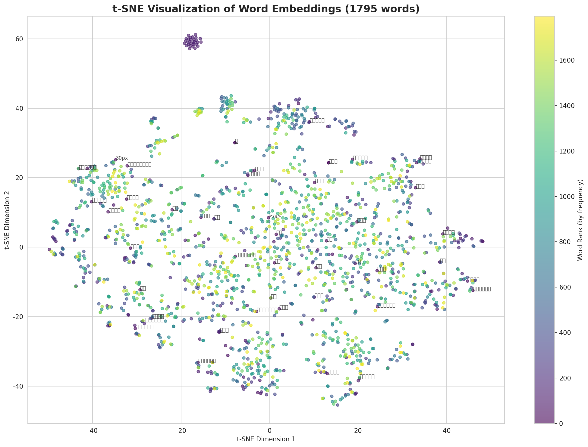
t-SNE Words	2D word embedding visualization
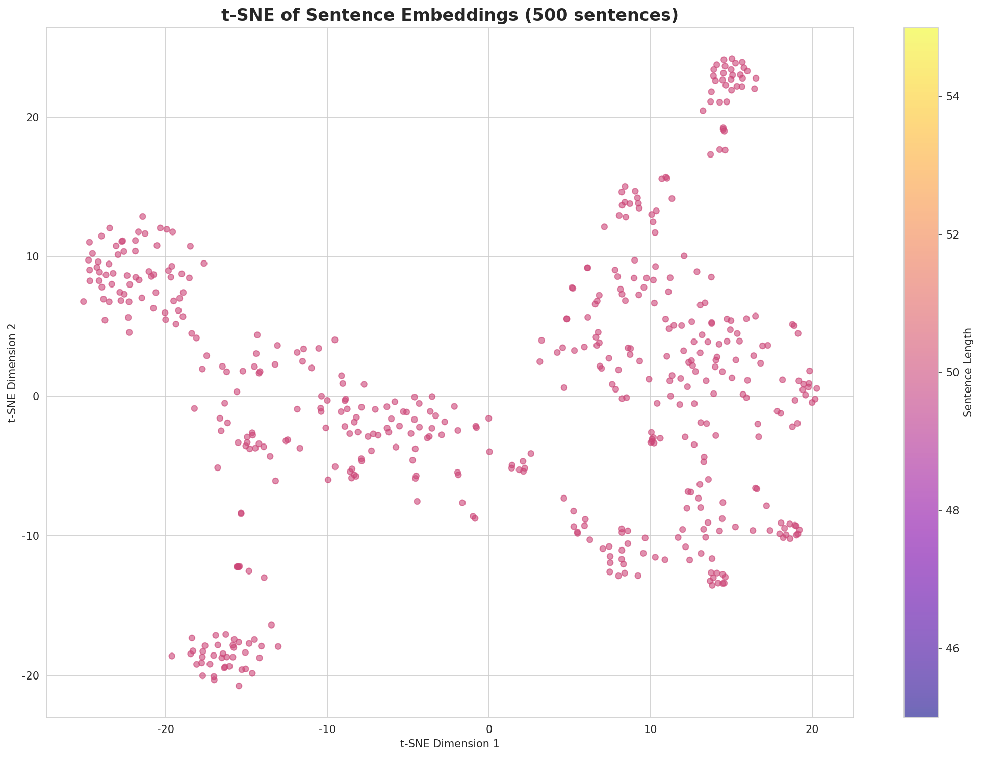
t-SNE Sentences	2D sentence embedding visualization
Position Encoding	Encoding method comparison
Model Sizes	Storage requirements
Performance Dashboard	Comprehensive performance overview

---

About This Project

Data Source

Models trained on wikipedia-monthly - a monthly snapshot of Wikipedia articles across 300+ languages.

Project

A project by Wikilangs - Open-source NLP models for every Wikipedia language.

Maintainer

Omar Kamali - Omneity Labs

Citation

If you use these models in your research, please cite:

@misc{wikilangs2025,
  author = {Kamali, Omar},
  title = {Wikilangs: Open NLP Models for Wikipedia Languages},
  year = {2025},
  doi = {10.5281/zenodo.18073153},
  publisher = {Zenodo},
  url = {https://huggingface.co/wikilangs}
  institution = {Omneity Labs}
}

License

MIT License - Free for academic and commercial use.

Links

• 🌐 Website: wikilangs.org
• 🤗 Models: huggingface.co/wikilangs
• 📊 Data: wikipedia-monthly
• 👤 Author: Omar Kamali
• 🤝 Sponsor: Featherless AI

---

Generated by Wikilangs Models Pipeline

Report Date: 2026-01-03 16:33:24